
Is 16GB VRAM Enough for Serious Local LLM Work?
Table of Contents
16GB of dedicated GPU memory supports serious local LLM work when your model, context, and runtime fit together. Loading the weights proves only the first requirement. A useful setup also needs enough memory for your working conversation and enough speed to finish your task.
Use Qwen3.8 27B as a worked example for budgeting a single-user coding or document workflow. Start with the context your task needs, then choose weights and runtime settings which fit the remaining memory. Hardware specifications and model sources were checked on October 7, 2026.
Key Takeaways
- Reserve memory for context before choosing a quantization.
- Measure prompt processing separately from output speed.
- Disable unused vision support and test an 8-bit KV cache.
- Compare the exact GPU, backend, model file, and prompt length.
- Calculate ownership savings from your workload and provider bill.
For the budgeting exercise, you need your runtime’s memory log, exact model filename, and a representative task. Allow about 20 minutes for setup and recording results, plus inference time. Difficulty is intermediate.
Match Memory to Work
16GB suits a workload whose weights, active context, and temporary allocations stay within available GPU memory. Your required context depends on the task. A short document summary and a coding agent reading dozens of files need different budgets.
| Workload | First sizing question |
|---|---|
| Short chat or drafting | Does the model meet your quality target? |
| Document analysis | Do the source text and answer fit together? |
| Coding agent | How much context do files and tool results consume? |
| Concurrent requests | How much cache does each active session need? |
A configured window differs from an occupied window. A benchmark with a 64K limit and a short prompt does not measure generation after 55K tokens of conversation. Test near your expected session length before choosing hardware.
Why the Model Fits
Quantization stores weights with fewer bits. Bartowski’s Qwen3.8 27B file table lists Q4_K_M at 17.44 GB, already beyond a 16 GiB device’s approximately 17.18 billion bytes before runtime memory.
ISTA-DASLab’s GSQ-RCO model card lists IQ3_S at 11.8 GB. Its method assigns different precision to different tensors within a size budget. The optional MTP version adds about 0.35 GB, while the vision projector adds about 0.9 GB.
| Published benchmark | BF16 / IQ3_S score |
|---|---|
| AIME25 | 100.00 / 100.00 |
| LiveCodeBench v6 | 85.71 / 85.71 |
| GPQA-Diamond | 89.90 / 89.39 |
The lab calls this operating point “task-lossless.” These selected results support a narrow comparison. They do not prove identical answers, equal long-context retrieval, or equal reliability across your coding tasks. Test the compressed model against your own acceptance criteria.
Count the Cache
The KV cache stores attention keys and values for tokens already processed. Your prompt, tool output, and generated answers consume context. Some runtimes allocate cache capacity at startup, so displayed memory need not grow with every message.
Qwen’s configuration specifies 64 layers, with full attention every fourth layer, four KV heads, and a head dimension of 256. For those 16 full-attention layers, the calculated FP16 cache cost is:
16 layers × 4 KV heads × 256 elements × 2 (K and V) × 2 bytes
= 65,536 bytes per token
= 64 KiB per token
This calculation excludes recurrent state, alignment, temporary buffers, and speculative decoding allocations. Other architectures need different calculations.
| Occupied tokens | FP16 full-attention cache |
|---|---|
| 32,768 | 2 GiB |
| 65,536 | 4 GiB |
| 131,072 | 8 GiB |
| 262,144 | 16 GiB |
Here, KiB and GiB use powers of 1024. Model download sizes use decimal GB. Mixing the units distorts the remaining budget.
Budget Your Available Context
Two settings free memory for longer text sessions: remove an unused vision projector and reduce cache precision. Calculate their effect against your loaded model and runtime allocations.
Use this worked example, with every allocation expressed in decimal GB. The 1.0 GB reserve below is a planning assumption, not a universal runtime default.
| Allocation | Vision on / vision off |
|---|---|
| Physical 16 GiB capacity | 17.180 / 17.180 GB |
| Model weights | 11.800 / 11.800 GB |
| Optional MTP head | 0.350 / 0.350 GB |
| Vision projector estimate | 0.930 / 0 GB |
| Assumed other allocations | 1.000 / 1.000 GB |
| Left for growing cache | 3.100 / 4.030 GB |
At 65,536 bytes per token, 3.100 GB holds about 47,300 tokens. With vision disabled, ideal 8-bit storage would use 32,768 bytes per token and hold about 123,000 tokens.
Real q8_0 storage includes block scales. At 34 bytes per 32 values, this example needs about 34,816 bytes per token, reducing the estimate to roughly 115,700. Additional allocations reduce the result further. Around 110K is therefore a plausible planning result under these assumptions, not a guaranteed setting.
The remaining context must cover both input and output. With a 65,536-token window, an illustrative 30,000-token initial prompt and an 8,192-token output allowance leave 27,344 tokens for files, tool results, and conversation. The initial prompt budget is an example. Measure your own tools and instructions.
Settings Worth Testing
The llama.cpp server documentation documents separate key and value cache types, automatic projector loading, and parallel slots. For a text-only workload, test vision disabled, q8_0 for both cache types, and one slot. Use a modest context first.
Record the resulting allocations before increasing context. Cache quantization needs support from your selected architecture and backend. Test answer quality after changing precision. Keep a working configuration for comparison.
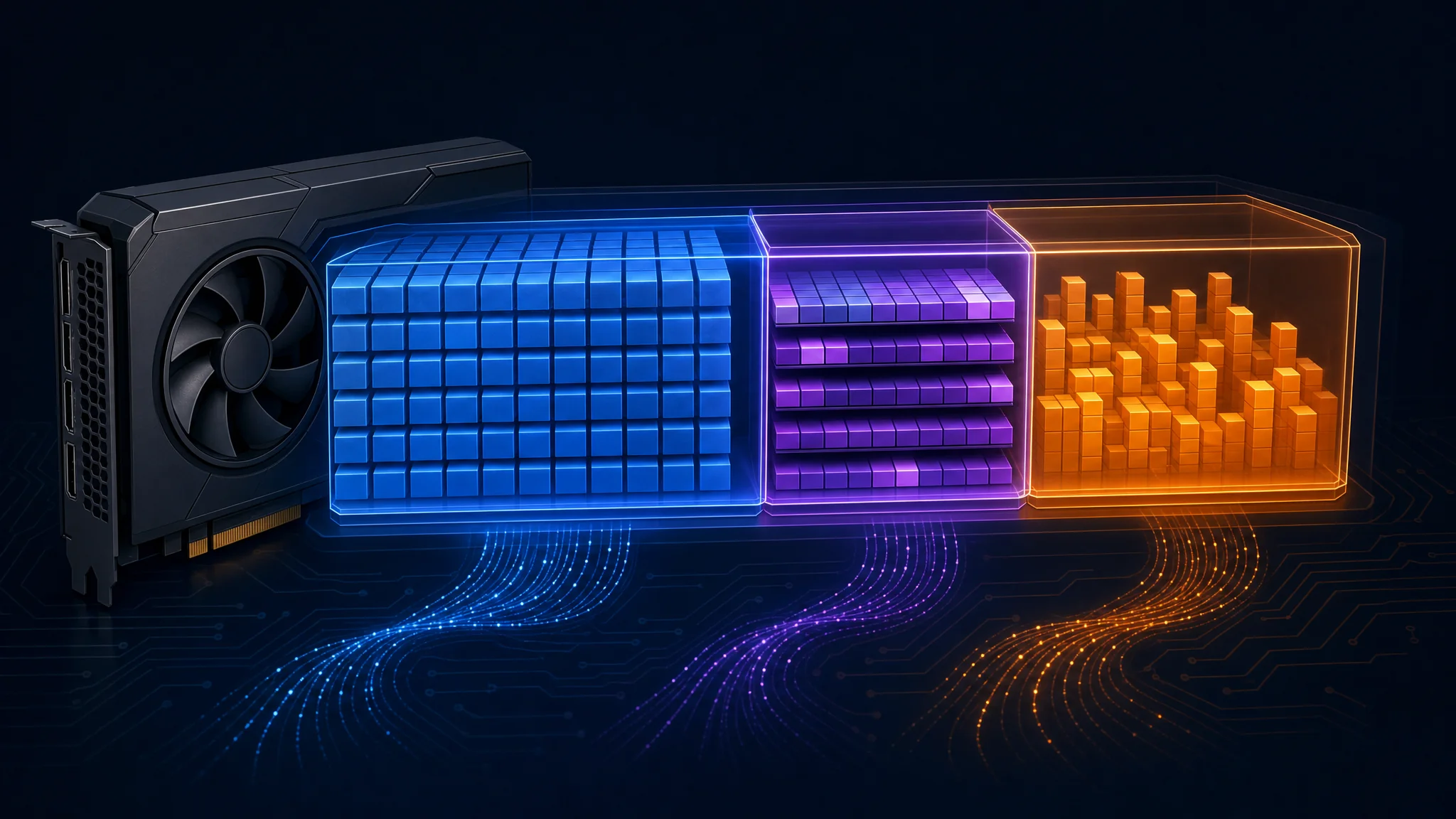
Blue represents weights, purple represents context cache, and orange represents runtime allocations. Sizes are illustrative
Why Speeds Differ
A 16GB label describes capacity. Throughput also depends on memory bandwidth, compute kernels, active context, offload, batching, and speculative decoding.
| Cause | What to inspect |
|---|---|
| CPU or RAM offload | Loaded layer placement and cache location |
| Long context | Occupied tokens during the measurement |
| Backend differences | Runtime commit, driver, and kernel path |
| Speculative decoding | Accepted drafts and extra allocations |
For a dense model generating one token at a time, memory bandwidth divided by resident weight bytes gives a rough bandwidth-only estimate. At 448 GB/s and 11.8 GB of weights, the quotient is about 38 tokens per second. Cache reads and computation add work, while speculative decoding and batching change the assumptions.
Do not treat this quotient as a universal upper bound. A higher reported output rate does not automatically invalidate a benchmark. Check whether one target-model pass accepted multiple draft tokens.
Multi-token prediction, or MTP, needs a compatible model and runtime. Compare enabled and disabled runs at both short and long occupied context. Extra weights and draft state consume memory, but no universal rule requires disabling MTP after 32K tokens.
Measure the First Reply
Prefill processes the prompt before generation. Decode produces the answer. A fast decode result hides a slow first response when a task begins with a large uncached prompt.
Divide uncached prompt tokens by measured prefill throughput to estimate prompt-processing time. For a fresh 30,000-token prompt, two illustrative rates produce these waits:
| Example prompt rate | Calculated processing time |
|---|---|
| 750 tokens/s | 40 seconds |
| 150 tokens/s | 200 seconds |
These examples describe processing time, excluding model loading and request overhead. Prompt length, batch size, model format, and backend affect your measured rate.
Measure a cold request and a continuation with a reusable prefix separately. Prefix reuse avoids processing some repeated input. Record time to first token alongside decode rate and total task duration.
Compare Complete GPU Setups
Compare purchase price, usable memory, bandwidth, and the software path together. A lower-priced card loses its advantage if your workload requires unsupported features or takes longer than your latency target.
| 16GB desktop card | Memory bandwidth |
|---|---|
| RX 9060 XT | 320 GB/s |
| RTX 5060 Ti | 448 GB/s |
| RX 9070 | 640 GB/s |
| RX 9070 XT | 640 GB/s |
AMD’s RX 9070 specifications and RX 9070 XT specifications confirm their 16GB capacity and up-to-640 GB/s bandwidth. The 640-to-448 comparison yields about 43% more theoretical bandwidth. A 43% inference improvement does not follow from those specifications.
Choose from benchmarks using your intended model and backend. For short prompts and sustained generation, decode performance deserves more weight. For repository analysis, prioritize cold prefill, long-context speed, and successful task completion. Check available software before buying either vendor.
Macs and Laptop Labels
A 16GB Apple silicon Mac shares memory among the CPU, GPU, operating system, and applications. A discrete 16GB GPU has dedicated video memory alongside system RAM. These capacities do not describe equivalent model budgets.
Apple exposes a recommended GPU working-set size . Inspect your runtime’s reported allowance and system memory pressure. Leave room for macOS and your other applications instead of budgeting the entire shared pool for inference.
For laptops, check the manufacturer’s exact SKU, dedicated memory, GPU power limit, and cooling. NVIDIA’s RTX 5060 family page lists desktop RTX 5060 Ti memory variants. A family name alone does not establish 16GB, and desktop results do not establish laptop throughput.
Does Ownership Pay?
Ownership pays financially when avoided hosting charges exceed operating costs and recover the hardware purchase. Start with an output-only example: a $789 card, 35 output tokens/s, 180W during generation, $0.18/kWh electricity, and $2.95 per million hosted output tokens. These are illustrative inputs. Replace them with your purchase quote, measured power, electricity rate, and provider pricing.
Hours per million output tokens = 1,000,000 ÷ 35 ÷ 3,600 = 7.94
Electricity per million = 7.94 × 0.180 kW × $0.18/kWh = $0.257
Savings per million = $2.95 - $0.257 = $2.693
Break-even output = $789 ÷ $2.693 = 293 million tokens
Continuous generation time = 293 × 7.94 ÷ 24 = about 97 days
At eight hours of uninterrupted generation per day, the same calculation takes about 291 days. Eight hours with an assistant open is different from eight hours generating tokens.
At a hosted output price of $0.16 per million, local electricity in this scenario already costs more than hosting. There is no positive output-only break-even point under these assumptions.
Use the selected provider’s current OpenRouter model pricing , including input and cached-input charges. Measure whole-system energy, including prefill. Add upgrades, idle energy, maintenance, and expected resale value. Compare accepted work, since retries and quality differences change cost per task.
When to Add Memory
Move beyond 16GB when your measured workload exceeds available context at acceptable quality and latency. Daily long agent sessions, concurrent requests, or higher-precision weights make larger capacity useful.
Two 16GB cards require explicit runtime support. They do not become one transparent 32GB allocation. Each device needs buffers, and communication uses the host’s interconnect.
| Split strategy | Main tradeoff |
|---|---|
| Layer split | Different layers occupy different devices |
| Tensor or row split | Work within layers adds communication |
| CPU plus GPU | More capacity with a different latency profile |
A second card deserves consideration when your motherboard, power supply, cooling, and backend already support the plan. Compare complete system cost with a larger single GPU. The 32GB Qwen hardware guide covers those alternatives.
Troubleshooting and Next Steps
If loading fails, lower context and inspect allocations. If speed falls during a session, check occupied context and CPU offload. If the first response stalls, measure cold prefill. If tool use breaks after compression, compare the same task with a higher-precision model.
Save one repeatable test containing your normal instructions, files, and tool outputs. Record model revision, runtime version, cache precision, occupied context, peak memory, first-token latency, decode speed, and whether the task passed. Repeat near your longest expected session.
Use the local model and context guide to compare smaller alternatives. Choose the smallest model meeting your quality requirements, then reserve enough memory for the complete task. Under those conditions, 16GB is a useful workstation target.

Related Posts